Grafana heatmaps with IRONdb have landed

GrafanaCon EU 2018 Recap

A couple weeks ago at GrafanaCon EU 2018 we announced the beta release of the IRONdb Data Source for Grafana. We’ve continued to make improvements to some features, such as the heatmap visualization of histogram data. In this blog post, we’ll show you how to use the IRONdb data source to produce these visualizations. We will start with the assumption that you already have IRONdb up and running; if not, the installation instructions are here. If you don’t want to install IRONdb, and instead want to try out the free hosted IRONdb version on Circonus, just keep reading to see the hosted example; we got you covered!

Data Source Installation

The first order of business is to get the data source installed. You’ll need Grafana v5.0 or 4.6.3 installed as a prerequisite, as it contains a number of updates needed for rendering the heatmap visualization. The IRONdb data source can be found here on GitHub. As with most Grafana plugins, the code is installed in /var/lib/grafana/plugins, and a server restart makes the data source available in the UI. Follow the data source configuration instructions, and you should have the IRONdb datasource installed on the Grafana host.

Data Source Configuration

Hosted or Standalone

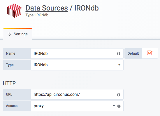
Your data source should look something like this; note that this is an example using the Circonus API (URL is set to https://api.circonus.com). If you don’t want to install IRONdb, you can create a Circonus account, grab an API token, and setup a hosted instance. Select IRONdb for the Type field under settings. Enter your IRONdb cluster url in the URL field (https://api.circonus.com for hosted, something like http://localhost:8112 for standalone). You’ll want proxy set under the Access field, since direct mode is not supported yet (this means requests to IRONdb are proxied through Grafana).

Auth and Advanced HTTP Settings

No changes are needed here from the default.

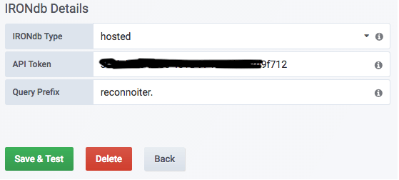
IRONdb Details

The rest of the configuration is specifying hosted or standalone under the installation type, and entering in the API Token.

For standalone IRONdb installation:

• Set the IRONdb Type field to standalone.
• Enter the Account ID to the value set in your irondb.conf file.
• Set the Query Prefix field to the root value of your metrics namespace for the metrics selector.

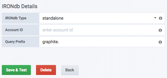
For hosted IRONdb installation:

• Set the IRONdb Type field to hosted.
• Enter the API Token from the API Token Page in your Circonus account.
• You will not need to make any change to the Query Prefix setting unless you are collecting your own custom metrics (like via Statsd).

Save & Test

Click to save the configuration and test the datasource; if it is working, you’ll see the “Data source is working” status message. If not, revisit the values you entered. Feel free to reach out to us at the Circonus Labs Slack #irondb channel if you have questions or problems you can’t resolve.

Collecting Histogram data

If you are an existing IRONdb user who has histogram metrics already available, you can go to the next step. If not, you’ll need to get histogram data into your instance. To generate a meaningful heatmap, you’ll likely want to be using data that represents latency or a duration, such as HTTP request duration.

For standalone IRONdb installations, see the IRONdb documentation on how to write histogram metrics.

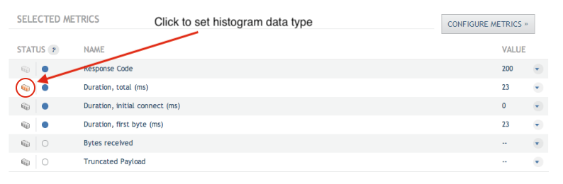
For hosted IRONdb installations, modify the metric type on an existing check you have (Integrations -> Checks) by clicking the histogram icon.

Creating the Heatmap Panel

Panel Creation

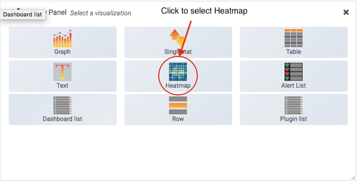
In your Grafana instance, click the + sign on the left nav, then select Heatmap from the grid.

Data Source Selection

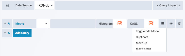
Select Edit at the top of the panel, and then under the Metrics tab, select your IRONdb data source from the drop down. Then to create a new metric, click the Histogram and CAQL boxes, and click the hamburger menu to the right and select Toggle Edit Mode.

Add Metrics

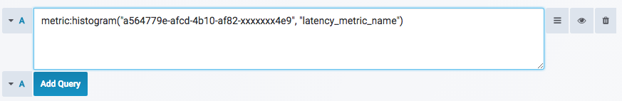
Now enter the check uuid and the metric name in the following CAQL (Circonus Analytics Query Language) format:

metric:histogram("<check_uuid>", "<metric_name>")

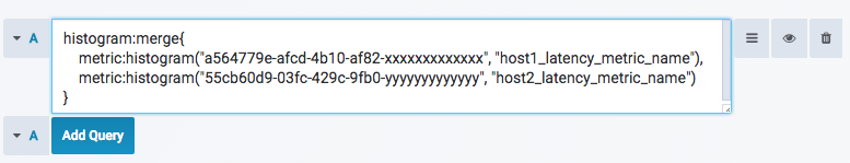
You can also merge multiple histograms metrics. If the upper left of the panel shows a red exclamation point, click the Query Inspector to debug the issue. Again, feel free to reach out to us at the Circonus Labs Slack #irondb channel if you don’t see data – this step isn’t always easy to get right the first time.

histogram:merge{
    metric:histogram("<check_uuid>", "<metric1_name>"),
    metric:histogram("<check_uuid>", "<metric2_name>") 
}

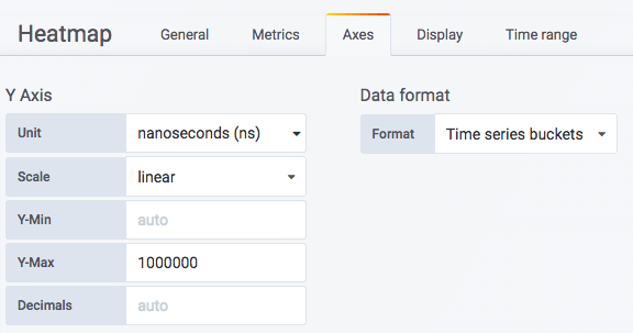
Setup Axes, Data format, and Colors

Select Time series buckets for Data Format, and select a Y-Max value so that you can see data on your display on the right scale.

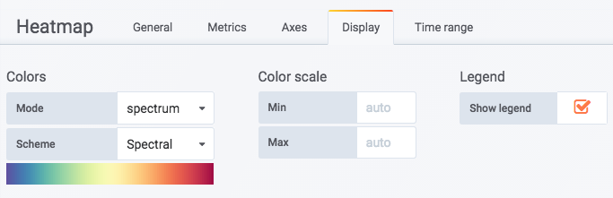
On the Display tab, select spectrum for Mode, and Spectral for Scheme. Click the Show legend box to display the legend and range

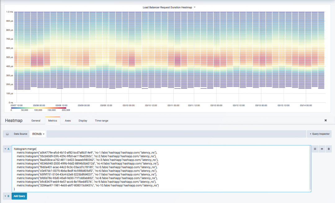
Let there be data!

At this point you should see a display something like this. There is a wealth of data encoded in this visualization of load balancer request latency. The band of red centers around the median response time of 500 nanoseconds, and is quite consistent across the map. This is an excellent visualization of the health of services, and is the D component in our RED dashboard. One thing to note here is that you can display the aggregate performance of an entire cluster, which is something that you can’t do with most other TSDB based tools. Other implementations can give you quantiles for individual hosts, but unless you are storing the telemetry data as a histogram (vs a quantile), you can’t calculate the cluster wide quantiles.

Other graphs

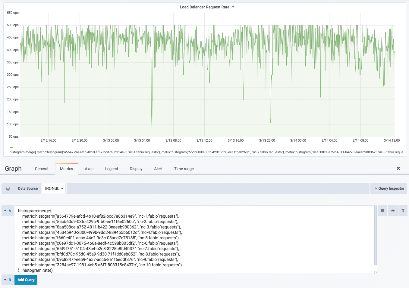
You can also display standard line graphs that have been the mainstay of monitoring displays. Here is a graph of load balancer request rates. I used the following CAQL statements to generate this by taking the rate of the requests serviced by each load balancer. Note that this is done on IRONdb and not in Grafana because we are using CAQL. We can still use the is_rate() function with the metric selector, but this is more efficient.

histogram:merge{
    metric:histogram("<check_uuid>", "<metric1_requests>"),
    metric:histogram("<check_uuid>", "<metric2_requests>"),
    metric:histogram("<check_uuid>", "<metric_n_requests>")
} | histogram:rate()

Metrics Selector

The regular Grafana metrics selector is also available with the IRONdb data source, you can select metrics via this standard interface. Leave the CAQL box unchecked for now, that’s for manually specifying the queries shown above.

Take it for a spin

We hope you enjoyed the walk through of the capabilities of our IRONdb Data Source. We’ll be adding some cool new features to this plugin over the next few months. You can keep up to date with the latest on this data source by following IRONdb on Twitter.