This two-part series examines the technical challenges of Time Series Databases (TSDBs) at scale. Like relational databases, TSDBs have certain technical challenges at scale, especially when the dataset becomes too large to host on a single server. In such a case you usually end up with a distributed system, which are subject to many challenges including the CAP theorem. This first half focuses on the challenges of data storage and data safety in TSDBs.
What is a Time Series Database?
Time series databases are databases designed to tracks events, or “metrics,” over time. The three most often used types of metrics (counters, gauges, and distributions) were popularized in 2011 with the advent of statsd by Etsy.
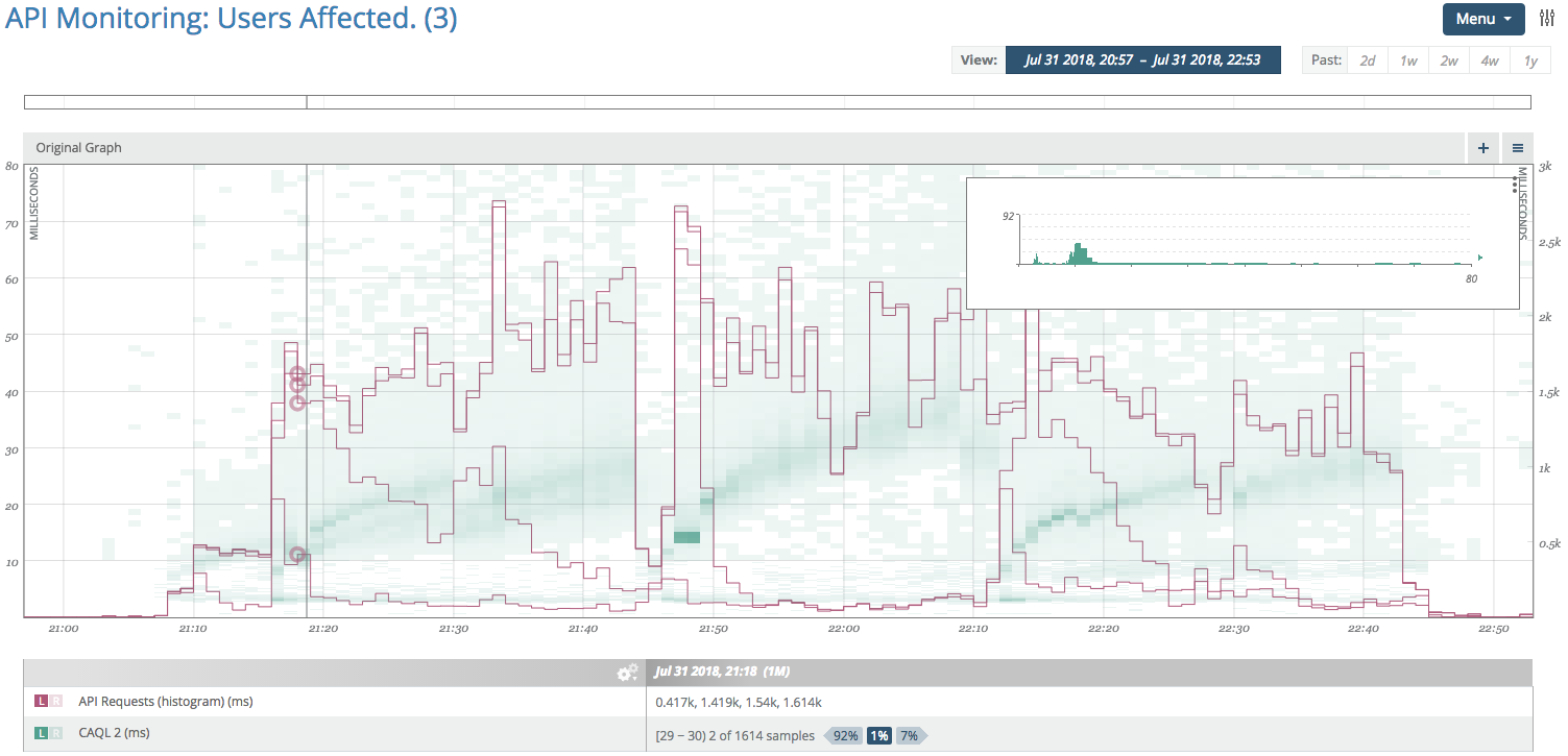
Time Series graph of API response latency median, 90th, and 99th percentiles.
The design goals of a TSDB are different from that of an RDBMS (relational database management systems). RDBMSs organize data into tables of columns and rows, with unique identifiers linking together rows in different tables. In contrast, TSDB data is indexed primarily by event timestamps. As a result, RDBMSs are generally ill-suited for storing time series data, just as TSDBs are ill-suited for storing relational data.
TSDB design has driven in large part by industry as opposed to academic theory. For example, PostgreSQL evolved from academia to industry, having started as Stonebraker’s Ingres (Post Ingres). But, sometimes ideas flow in the other direction, with industry informing academia. Facebook’s Gorilla is an example of practitioner driven development that has become noted in academia.
Data Storage
Modern TSDBs must be able to store hundreds of millions of distinct metrics. Operational telemetry from distributed systems can generate thousands of samples per host, thousands of times per second, for thousands of hosts. Historically successful storage architectures now face challenges of scale orders of magnitude higher than they were designed for.
How do you store massive volumes of high-precision time-series data such that you can run analysis on them after the fact? Storing averages or rollups usually won’t cut it, as you lose fidelity required to do a mathematically correct analysis.
From 2009 to 2012, Circonus stored time series data in PostgreSQL. We encountered a number of operational challenges, the biggest of which was data storage volume. A meager 10K concurrent metric streams, sampling once every 60 seconds, generates 5 billion data points per year. Redundantly storing these same streams requires approximately 500GB of disk space. This solution scaled, but the operational overhead for rollups and associated operations was significant. Storage nodes would go down, and master/slave swaps take time. Promoting a read only copy to write master can take hours. An unexpectedly high amount of overhead, especially if you want to reduce or eliminate downtime — all to handle “just” 10K concurrent metric streams.
While PostgreSQL is able to meet these challenges, the implementation ends up being cost prohibitive to operate at scale. Circonus evaluated other time series storage solutions as well, but none sufficiently addressed the challenges listed above.
So how do we store trillions of metric samples?
TSDBs typically store numeric data (i.e. gauge data) for a given metric as a set of aggregates (average, 50th / 95th / 99th percentiles) over a short time interval, say 10 seconds. This approach can generally yield a footprint of three to four bytes per sample. While this may seem like an efficient use of space, because aggregates are being stored, only the average value can be rolled up to longer time intervals. Percentiles cannot be rolled up except in the rare cases where the distributions which generated them are identical. So 75% of that storage footprint is only usable within the original sampling interval, and unusable for analytics purposes outside that interval.
A more practical, yet still storage efficient approach, is to store any high frequency numeric data as histograms. In particular, log linear histograms, which store a count of data points for every tenth power in approximately 100 bins. A histogram bin can be expressed with 1 byte for sample value, 1 byte for bin exponent (factor of 10), and 8 bytes for bin sample count. At 10 bytes per sample, this approach may initially seem less efficient, but because histograms have the property of mergeability, samples from multiple sources can be merged together to obtain N increases of efficiency, where N is the number of sample sources. Log linear histograms also offer ability to calculate quantiles over arbitrary sample intervals, providing a significant advantage over storing aggregates.
Data is rolled up dynamically, generally at 1 minute, 30 minute, and 12 hour intervals, lending itself to analysis and visualization. These intervals are configurable, and can be changed by the operator to provide optimal results for their particular workloads. These rollups are a necessary evil in a high volume environment, largely due to the read vs write performance challenges when handling time series data. We’ll discuss this further in part 2.
Data Safety
Data safety is a problem common to all distributed systems. How do you deal with failures in a distributed system? How do you deal with data that arrives out of order? If you put the data in, will you be able to get it back out?
All computer systems can fail, but distributed systems tend to fail in new and spectacular ways. Kyle Kingsbury’s series “Call Me Maybe” is a great educational read on some of the more entertaining ways that distributed databases can fail.
Before developing IRONdb in 2011, Circonus examined the technical considerations of data safety. We quickly realized that the guarantees and constraints related to ACID databases can be relaxed. You’re not doing left outer joins across a dozen tables; that’s a solution for a different class of problem.
Can a solution scale to hundreds of millions of metrics per second WITHOUT sacrificing data safety? Some of the existing solutions could scale to that volume, but they sacrificed data safety in return.
Kyle Kingsbury’s series provides hours of reading detailing the various failure modes experienced when data safety was lost or abandoned.
IRONdb uses OpenZFS as its filesystem. OpenZFS is the open source successor to the ZFS filesystem which was developed by Sun Microsystems for the Solaris operating system. OpenZFS compares the checksums of incoming writes to checksums of the existing on-disk data and avoid issuing any write I/O for data that has not changed. It supports on the fly LZ4 compression of all user data. It also provides repair on reads, and the ability to scrub file system and repair bitrot.
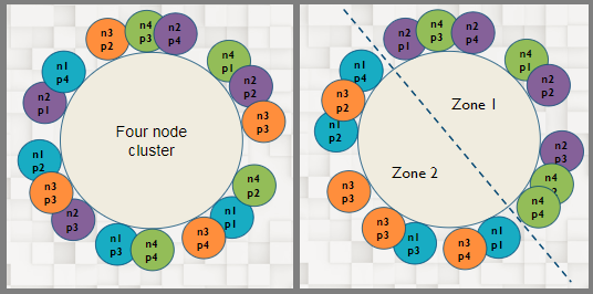
To make sure that whatever data is written to the system can be gotten out, IRONdb writes data to multiple nodes. The number of nodes is dependent on the replication factor, which is 2 in this example diagram. On each node, data is mirrored to multiple disks for redundancy.
The CAP theorem says that since all systems experience network partitions, they will sacrifice either availability or consistency. The effects of the CAP theorem can be minimized, as shown in Google’s Cloud Spanner blog post by Eric Brewer (the creator of the CAP theorem). But in systems that provide high availability, it’s inevitable that some the data will be out of order.
Dealing with data that arrives out of order is a difficult problem in computing. Most systems attempt to resolve this problem through the use of consensus algorithms such as Raft or Paxos. Managing consistency is a HARD problem. A system can give up availability in favor of consistency, but this ultimately sacrifices scalability. The alternative is to give up consistency and present possibly inconsistent data to the end user. Again, see Kyle Kingsbury’s series above for examples of the many ways that goes wrong.
IRONdb tries to avoid these issues all together through the use of commutative operations. This means that the final result recorded by the system is independent of the order of operations applied. Commutative operations can be expressed mathematically by f(A,B) = f(B,A). This attribute separates IRONdb from pretty much every other TSDB.
The use of commutative operations provides the core of IRONdb’s data safety, and avoids the most complicated part of developing and operating a distributed system. The net result is improved reliability and operational simplicity, allowing operators to focus on producing business value as opposed to rote system administration.
There are a lot of other ways to try and solve the consistency problem. All have weaknesses and are operationally expensive. Here’s a comparison of known consensus algorithms used by other TSDBs:
| TSDB/Monitoring Platform | Solution to Consistency Problem |
|---|---|
| IRONdb | Avoids problem via commutative operations |
| DalmatinerDB | Multi-Paxos via Riak core |
| DataDog | Unknown, rumored to use Cassandra (Paxos) |
| Graphite (default without IRONdb) | None |
| InfluxDB | Raft |
| OpenTSDB | HDFS/HBase (Zookeeper’s Zab) |
| Riak | Multi-Paxos |
| TimescaleDB | Unknown, PostgreSQL based |
That concludes part 1 of our series on solving the technical challenges of TSDBs at scale. We’ve covered data storage and data safety. Next time we’ll describe more of the technical challenges inherent in distributed systems and how we address them in IRONdb. Check back for part 2, when we’ll cover balancing read vs. write performance, handling sophisticated analysis of large datasets, and operational simplicity.