This is the second half of a two-part series focusing on the challenges of Time Series Databases (TSDBs) at scale. This half focuses on the challenges of balancing read vs. write performance, data aggregation, large dataset analysis, and operational complexity in TSDBs.
Balancing Read vs. Write Performance
Time series databases are tasked with ingesting concurrent metric streams, often in large volumes. This data ultimately needs to be persisted to permanent storage, where later it can be retrieved. While portions of the ingest pipeline may be temporarily aggregated in memory, certain workloads require either write queuing or a high-speed data storage layer to keep up with high inbound data volumes.
Data structures such as Adaptive Radix Trees (ARTs) and Log-Structured Merge-trees (LSMs) provide a good starting point for in-memory and memory/disk indexed data stores. However, the requirement to quickly persist large volumes of data presents a conundrum of read/write asymmetry. The greater the capacity to ingest and store metrics, the larger the volume of data available for analysis, creating challenges for read-based data analysis and visualization.
Analyzing time-series data reveals an inherent constraint: one must be able to read data at an exponentially higher rate than it was ingested at. For example, retrieving a week’s worth of time-series data within a single second to support some type of visualization and analysis.
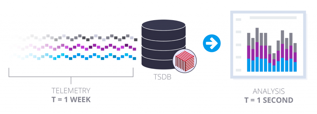
Read/write asymmetry of analyzing 1 weeks worth of time-series based telemetry data
How do you scale reads for large amounts of data in a non-volatile storage medium? The typical solution to this asymmetry is data aggregation — reducing the requisite volume of read data while simultaneously attempting to maintain its fidelity.
Data Aggregation
Data aggregation is a crucial component of performant reads. Many TSDBs define downsampling aggregation policies, storing distinct sampling resolutions for various retention periods. These aggregations can be asynchronously applied during ingestion, allowing for write performance optimizations. Recently ingested data is often left close to sample resolution, as it loses value when aggregated or downsampled.
These aggregations are accomplished by applying an aggregation function over data spanning a time interval. Averaging is the most common aggregation function used, but certain TSDBs such as IRONdb and OpenTSDB provide the ability to implement other aggregation functions such as max(), sum() , or histogram merges. The table below lists some well-known TSDBs and the aggregation methods they use.
| TSDB/Monitoring Platform | Solution to Consistency Problem |
|---|---|
| IRONdb | Automatic rollups of raw data after configurable time range |
| DalmatinerDB | DQL aggregation via query clause |
| Graphite (default without IRONdb) | In memory rollups via carbon aggregator |
| InfluxDB | InfluxQL user defined queries run periodically within a database, GROUP BY time() |
| OpenTSDB | Batch processed, queued TSDs, or stream based aggregation via Spark (or other) |
| Riak | User defined SQL type aggregations |
| TimescaleDB | SQL based aggregation functions |
| M3DB | User defined rollup rules applied at ingestion time, data resolution per time interval |
As mentioned in part one , histograms are useful in improving storage efficiency, as are other approximation approaches. These techniques often provide significant read performance optimizations. IRONdb uses log linear histograms to provide these read performance optimizations. Log linear histograms allow one to store large volumes of numeric data which can be statistically analyzed with a quantifiable error rates, in the band of 0-5% on the bottom of the log range, and 0-0.5% on the top of the log range.
Approximate histograms such as t-digest are storage efficient, but can exhibit error rates upwards of 50% for median quantile calculations. Uber’s M3DB uses Bloom filters to speed data access times, which exhibit single digit false positive error rates for large data sets in return for storage efficiency advantages. Efficiency versus accuracy tradeoffs should be understood choosing an approximation based aggregation implementation.
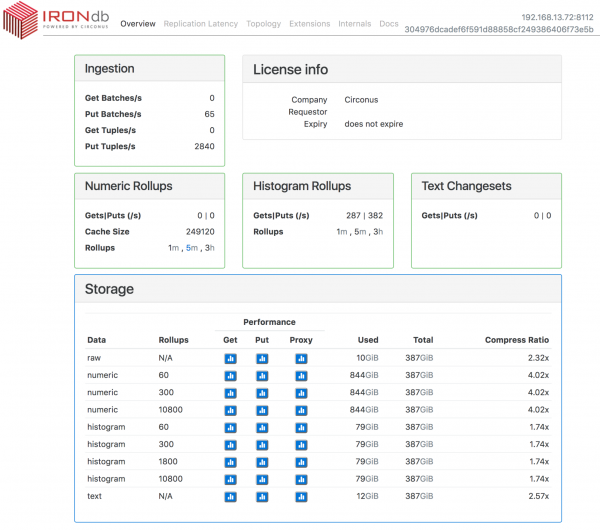
Default aggregation policies, broken down by type, within IRONdb
It is important to note a crucial trade-off of data aggregation: spike erosion . Spike erosion is a phenomenon exhibited where visualizations containing aggregated data over wide intervals display lower interval sample maximums. This occurs in scenarios where averages are used as the aggregation function (which is the case for most TSDBs). The use of histograms as a data source can guard against spike erosion by allowing application of a max() aggregation function for intervals. However, a histogram is significantly larger to store than a rollup, so that accuracy comes at a cost.
Analysis of Large Datasets
One of the biggest challenges with analyzing epic data sets is that moving or copying data for analysis becomes impractical due to the sheer mass of the dataset. Waiting days or weeks for these operations to complete is incompatible with the needs of today’s data scientists.
The platform must not only handle large volumes of data, but also provide tools to perform internally consistent statistical analyses. Workarounds won’t suffice here, as cheap tricks such as averaging percentiles produce mathematically incorrect results. Meeting this requirement means performing computations across raw data, or rollups that have not suffered a loss of fidelity from averaging calculations.
Additionally, a human-readable interface is required, affording users the ability to query and introspect their datasets in arbitrary ways. Many TSDBs use the “in place” query approach. Since data cannot be easily moved at scale, you have to bring the computation to the data.
PromQL, from Prometheus, is one example of such a query language. IRONdb, on the other hand, uses the Circonus Analytics Query Language (CAQL), which affords custom user-definable functions via Lua.
Anyone who has worked with relational databases and non-procedural languages has experienced the benefits of this “in place” approach. It is much more performant to delegate analytics workloads to resources which are computationally closer to the data. Sending gigabytes of data over the wire for transformation is grossly inefficient when it can be reduced at the source.
Operational Complexity
Operational complexity is not necessarily a “hard problem,” but is sadly an often ignored one. Many TSDBs will eventually come close to the technical limits imposed by information theory. The primary differentiator then becomes efficiency and overall complexity of operation.
In an optimal operational scenario, a TSDB could automatically scale up and down as additional storage or compute resources are needed. Of course, this type of idealized infrastructure is only present on trade-show marketing literature. In the real world, operators are needed, and generally some level of specialized knowledge is required to keep the infrastructure properly running.
Let’s take a quick look at what’s involved in scaling out some of the more common TSDBs in the market:
| TSDB/Monitoring Platform | Solution to Consistency Problem |
|---|---|
| IRONdb | Generate new topology config, kick off |
| DalmatinerDB | Rebalance via REST call |
| Graphite (default without IRONdb) | Manual, file based. Add HAProxy or other stateless load balancer |
| InfluxDB | Configure additional name and/or data nodes |
| OpenTSDB | Expand your HBASE cluster |
| Riak | RiakTS cluster tools |
| TimescaleDB | Write clustering in development |
| M3DB | M3DB Docs |
There are other notable aspects of operational complexity. For example, what data protection mechanisms are in-place?
For most distributed TSDBs, the ability to retain an active availability zone is sufficient. When that’s not enough (or if you don’t have an online backup), ZFS snapshots offer another solution. There are, unfortunately, few other alternatives to consider. Typical data volumes are often large enough that snapshots and redundant availability zones are the only practical options.
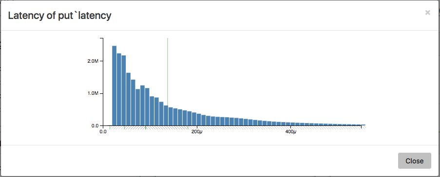
A key ingestion performance visualization for IRONdb, a PUT latency histogram, shown as it appears within IRONdb’s management console
Another important consideration is observability of the system, especially for distributed TSDBs. Each of the previously mentioned options conveniently expose some form of performance metrics, providing a way through which one may monitor the health of the system. IRONdb is no exception, offering a wealth of performance metrics and associated visualizations such that one can easily operate and monitor it.
Conclusion
There are a number of factors to consider when either building your own TSDB, or choosing an open-source or commercial option. It’s important to remember that your needs may differ from those of Very Large Companies. These companies often have significant engineering and operations resources to support the creation of their own bespoke implementations. However, these same companies often have niche requirements that prevent them from using some of the readily available options in the market, requirements that smaller companies simply don’t have.
If you have questions about this article, or Time Series Databases in general, feel free to join our slack channel and ask us.